

Learning UQLab by example
We made a significant effort to provide UQLab users with a number of examples that can be used to gradually learn all the features of the software.
Each example is especially prepared to provide users with enough experience and background to develop their own applications in no time. The examples are divided into different categories, as explained below.
Contents
-
Surrogate model benchmarking
-
Stochastic polynomial chaos
-
Generalized lambda models
-
Random fields
-
Stochastic spectral embedding
-
HPC dispatcher
-
Reliability-based design optimization
-
Bayesian inversion
-
UQLink
-
Support vector machines
-
Probabilistic input
-
Deterministic and stochastic models
-
Polynomial chaos expansions
-
Kriging
-
Polynomial chaos-Kriging
-
Low-rank approximations
-
Sensitivity analysis
-
Reliability analysis
Surrogate Model Benchmarking
Benchmarking surrogate models against the state-of-the-art on suitable case studies is an important step for their validation.
The Benchmarking module provides extensive facilities to quantitatively assess, compare and visualize the performance of surrogate models across different usage scenarios.


Dispatch expensive computations to a remote machine, while keeping the Matlab session synchronized.


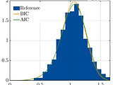
Stochastic Polynomial Chaos Expansions
Stochastic polynomial chaos expansions (SPCE) represent a novel class of surrogate models, designed to efficiently and accurately approximate the statistical behavior of non-deterministic models, or stochastic simulators.
SPCE does not require the presence of replications for training, and can reproduce even multi-modal stochastic responses.


Generalized Lamda Models
Capitalizing on the highly flexible family of generalized lambda distributions, generalized lambda models (or GLaM in brief) can reproduce the stochastic behavior of complex stochastic simulators.
While limited to unimodal stochastic responses, GLaMs can directly provide (semi-)analytical expressions for conditional responses, quantiles, and many other desirable features. They can be trained both on datasets with replications, and on datasets without replications.


Random Fields
Random fields are used in many uncertainty quantification problems to model random parameters that vary in space and/or time.
UQLab offers an intuitive way to define a random field using its key properties, discretize it and eventually sampling from it.

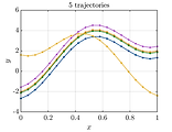
Learn how to specify the properties of a random field and draw samples from it.

Build a conditional random field using EOLE and compare its mean to a Kriging predictor

Build a lognormal random field and map its samples into an equivalent random field with different marginals

Lean how to use different discretization schemes to build a two-dimensional random field.

Lean how to use a random field in conjunction with surrogate modeling to solve a complex problem.
High-performance computing (HPC) dispatcher
Distributed computing resources give users possibilities to scale up, speed up, or offload UQLab computations typically running on their personal computers. The associated workflows, however, tend to be rather complex, from the submission of the computations to their retrieval.
The HPC dispatcher module of UQLab offers an interface between the user personal computers and common distributed computing resources (e.g. HPC clusters), to seamlessly set up, submit and retrieve parallel computation jobs directly within UQLab.


Stochastic spectral embedding
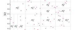
Stochastic spectral embedding is a novel metamodeling strategy that takes advantage of the global accuracy and fast convergence of PCE, while at the same time locally refining the expansion throughout the input domain.
The UQLab stochastic spectral embedding tool provides an effective tool to surrogate complex computational models with heterogeneous complexity accurately and efficiently.

Efficiently surrogate complex heterogeneous functions

Use SSE to surrogate a non-smooth, non-differentiable function
Surrogate a function that is mostly 0 in the input domain, except in a small region
Use SSE for multi-output models
Reliability-based design optimization
Reliability-based design optimization (RBDO) is a powerful tool for the design of structures under uncertainty. UQLab offers an intuitive way to set-up and solve RBDO problems using either state-of-the-art algorithms or custom solution schemes, which combine various reliability, optimization and surrogate modeling techniques.

Learn how to set up and solve a simple problem using state-of-the-art RBDO approaches.
Learn how to set up your own RBDO solution scheme by combining reliability and optimization techniques available in UQLab.


Learn how to use surrogate models to alleviate the computational burden of RBDO.
Bayesian inversion
Bayesian inversion is a powerful tool for probabilistic model calibration and validation. UQLab offers users an intuitive way to set up Bayesian inverse problems with customizable likelihood functions and discrepancy model options; and solve the problems with state-of-the art Markov Chain
Monte Carlo (MCMC) algorithms.

Learn how to set up and solve a Bayesian calibration problem using a simple model of beam deflection.


Learn how to solve the classical Bayesian linear regression problem, with known and unknown residual variance.

Learn how to calibrate a conceptual watershed model (HYMOD) using historical data.

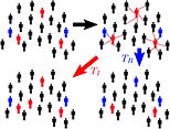
Learn how to calibrate a predator-prey model of lynx and hare populations with multiple model discrepancy options.

Learn how to set up and calibrate simultaneously multiple forward models of a simple beam.

Set up and use a custom user-defined likelihood function to model dependence between data points.

Compute the MAP estimator of the model parameters of a linear regression model.


Conduct a Bayesian inversion analysis with a surrogate model to reduce the overall computational time.

Deploy the recently developed SLE and SSLE sampling-free inversion strategies onto the beam calibration problem.
UQLink
UQLab allows one to easily define computational models involving a third-party software through a built-in universal "code wrapper".
After the wrapper has been configured through input/output text files and ad-hoc text marking and parsing, the corresponding computational model can be seamlessly integrated with any techniques available in other UQLab modules to create complex analyses in no time.

Link UQLab to a C code implementing
a simply supported beam then carry out a reliability analysis using AK-MCS.

Link UQLab to an Abaqus model of
a ten-bar truss then carry out
sensitivity and reliability analyses.

Link UQLab to OpenSees for
a pushover analysis of a two-story
one-bay structure.
Support vector machines
Support vector machines (SVM) belong to a class of machine learning techniques developed since the mid-'90s. In the context of uncertainty quantification, support vector machines for classification (SVC) can be used to build a classifier given an experimental design. They can be used for reliability analysis (a.k.a. rare events estimation). Support vector machines for regression (SVR) can be used as a metamodeling tool to approximate a black-box or expensive-to-evaluate computational model.
Classification (SVC)
UQLab offers a straightforward parametrization of a SVC model to be fitted on the data set at hand (e.g. a design of computer experiments): linear and quadratic penalization schemes, separable and elliptic kernels based on classical SVM kernels (linear, polynomial, sigmoid) and others (Gaussian, exponential, Matérn, user-defined). Different techniques including the span leave-one-out and the cross-validation error estimation methods as well as various optimization algorithms are available to estimate the hyperparameters.

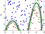
Learn how to select different kernel families through an introductory SVC example based on the Fisher’s iris data set.
Learn how to use the span estimate of the leave-one-out error or K-fold cross-validation as well as various optimization strategies.

Create an SVC model from existing data (a breast cancer data set).
Regression (SVR)
UQLab offers a straightforward parametrization of an SVR model to be fitted on the data set at hand (e.g., an experimental design):
L1- and L2-penalization schemes, separable and elliptic kernels based on classical SVM kernels (linear, polynomial, sigmoid) and others (Gaussian, exponential, Matérn, user-defined). Different techniques, including the span leave-one-out and the cross-validation error estimation methods, as well as various optimization algorithms, are available to estimate the hyperparameters.

Learn how to select different kernel families through an introductory SVR example.

Learn how to use the span estimate of the leave-one-out error or K-fold cross-validation as well as various optimization strategies.

Apply SVR to a computational model with multiple outputs.

Create an SVR model from existing data (the Boston housing data set).
Probabilistic Input
Whether the uncertainty sources are simple independent uniform variables or complex combinations of fancy marginals glued together by a copula, UQLab provides simple methods to define, sample or transform your input distributions. If the theoretical marginals and/or copulas are unknown and only data are available, uqlab provides the possibility to infer the unknown distributions from the data in a simple way.

Learn how to specify a random vector and draw samples using various sampling strategies.

Learn how to specify marginal distributions for the elements of a random vector and a Gaussian copula.

Learn how to specify marginal distributions for the elements of a random vector and a Pair copula.

Learn how to specify marginal distributions for the elements of a random vector and a (C- or D-) vine copula.

Learn how to group uncertain inputs into mutually independent subsets (blocks) via multiple copulas.


Learn how to infer the marginal distributions of an input from data.

Learn how to infer the copula of an input from data, and how to perform independence tests.
Basic modeling
UQLab allows one to simply define new computational models, either based on existing m-code files, function handles, or simple text strings.
After a computational model has been configured, it can be seamlessly integrated with any other technique to create complex analyses in no time.

Learn different ways to define a computational model.

Learn how to pass parameters to a computational model.

Learn how to handle models that return vector outputs instead of scalars.

Polynomial chaos expansions
Modern computational models are often expensive-to-evaluate. In the context of uncertainty quantification, where repeated runs are required,
only a limited budget of simulations is usually affordable. We consider a “reasonable budget” to be in the order of 50-500 runs.
With this limited number of runs, a polynomial surrogate may be built, which mimics the behavior of the true model at a close-to-zero computational cost. Polynomial chaos expansions are a particularly powerful technique which makes use of so-called orthogonal polynomials with respect to the input probability distributions.

Learn how to deploy various strategies to compute PCE coefficients.

Try out various methods to generate an experimental design (DOE) and compute PCE coefficients with least-square minimization.

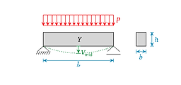
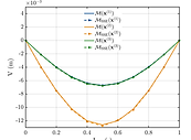
Apply sparse PCE for the estimation of the mid-span deflection of a simply supported beam subject to a uniform random load.

Apply sparse PCE to surrogate a model with multiple outputs.

Build a sparse PCE surrogate model from existing data.

Build a sparse PCE using polynomials orthogonal to arbitrary distributions

Apply the bootstrap method to estimate the local errors of PCE metamodel predictions.
Kriging
Kriging (Gaussian process modeling) considers the computational model as a realization of a Gaussian process indexed by the parameters
in the input space.
UQLab offers a straightforward parametrization of the Gaussian process to be fitted to the experimental design points: constant, linear, polynomial, or arbitrary trends, with separable and elliptic kernels based on different one-dimensional families (Gaussian, exponential, Matérn, or user-defined).
The hyperparameters can be estimated either using the Maximum-Likelihood or the Cross-Validation method using various optimization techniques (local and global). UQLab supports both interpolation and regression (Kriging with noisy model response) mode.

Learn how to select different correlation families through an introductory Kriging example.

Learn how to use maximum likelihood or leave-one-out cross-validation as well as various optimization strategies.

Learn how to specify various trend types.

Create a Kriging surrogate for a function with multiple input dimensions (the Branin-Hoo function).

Create a Kriging surrogate from existing data (the truss structure data set).

Create a Kriging surrogate from existing data (the Boston housing data set).

Apply Kriging to a computational model with multiple outputs.


Learn how to create a Gaussian process regression (GPR) model for model with noisy response.

Apply GPR to create a regression model for the Boston housing data set.

Polynomial Chaos-Kriging
Polynomial Chaos-Kriging (PC-Kriging) combines features from polynomial chaos expansions and Kriging in a single efficient surrogate.
A PC-Kriging model is effectively a universal Kriging model with a sophisticated trend based on orthogonal polynomials. By adopting advanced sparse polynomial chaos expansion techniques based on compressive sensing, PC-Kriging can effectively reproduce the global approximation behavior typical of PCE, while at the same time retaining the interpolatory characteristics of Kriging.
The PC-Kriging implementation in UQLab leverages on the PCE and Kriging modules, to provide a fully-configurable tool that is seamlessly integrated with the whole metamodeling tools offered by the platform.

Learn how to create a PC-Kriging surrogate of a simple one-dimensional function.

Learn how to create a PC-Kriging metamodel of a multi-dimensional function (the Ishigami function).

Apply PC-Kriging to a computational model with multiple outputs.

Create a PC-Kriging metamodel from existing data (the truss data set).
Low-rank approximations
Canonical low-rank polynomial approximations (LRA), also known as separated representations, have recently been introduced in the field of uncertainty quantification as a promising tool for effectively dealing with high-dimensional model inputs. The key idea is to approximate a response quantity of interest with a sum of a small number of appropriate rank-one tensors, which are products of univariate polynomial functions.
An important property of LRA is that the number of unknowns increases only linearly with the input dimension, hence making them a powerful tool to tackle high dimensional problems.
The LRA module in UQLab capitalizes on the PCE module to create low-rank representations, hence offering similar flexibility in terms of supported polynomial types.

Create a canonical low-rank tensor approximation of a simple engineering model.

Create a canonical low-rank tensor approximation of a highly non-linear function.

Create a canonical low-rank tensor approximation of a complex function.

Learn how to create a canonical low-rank tensor approximation of a model with multiple outputs.

Learn how to create a canonical low-rank tensor approximation from existing data (the truss data set).
Sensitivity analysis
Sensitivity analysis is a powerful tool to identify which variables contribute the most to the variability of the response of a computational model.
UQLab offers a wide selection of sensitivity analysis tools, ranging from sample-based methods (e.g., input/output correlation), linearization methods (e.g., perturbation analysis), screening methods (e.g., Morris' elementary effects), moment-independent method (e.g., Borgonovo indices), to the more advanced ANOVA- (ANalysis Of Variance) measures for independent (e.g., Sobol' indices) and dependent inputs parameters (e.g., ANCOVA indices).
The algorithms take advantage of the latest available sampling-based algorithms as well as some metamodel-specific techniques to extract the most accurate information based on relatively small sample size (e.g., polynomial chaos expansion- and low-rank-approximation-based Sobol' indices).

Apply various sensitivity analysis techniques to a benchmark problem (borehole function).

Learn how to obtain the Sobol' indices using either the sampling-based or the PCE/LRA-based methods.

Discover the amazing efficiency of
PCE-based Sobol' analysis on
a 100-dimensional example.

Apply sensitivity analysis techniques to model with multiple outputs.

Apply sensitivity analysis techniques to model with dependent inputs.
Reliability analysis
The reliability analysis (rare events estimation) module provides a set of tools to determine the probability that some criterion on the model response is satisfied, e.g., the probability of exceedance of some prescribed admissible threshold.
The reliability analysis module in UQLab comprises a number of classical techniques (e.g., FORM and SORM approximation methods,
classical Monte-Carlo Sampling (MCS), Importance Sampling, and Subset Simulation) as well as the more recent surrogate modeling-based methods (e.g., Adaptive Kriging Monte-Carlo simulation).
The reliability analysis module in UQLab also offers a modular framework that allows users to easily build active learning custom solution schemes
by combining a selection of surrogate models and reliability algorithms, learning function, and stopping criteria.
All the available algorithms take advantage of the high interoperability with the other modules of UQLab, hence making their deployment time-efficient

Learn how to apply all of the available reliability analysis algorithms on a classic linear example: the R-S case.

See how different simulation-based methods perform on a highly non-linear limit state function.

Apply several different algorithms in a high-dimensional, strongly non-linear test case.

Perform reliability analysis on a parallel system with the FORM method.

Compute the outcrossing rate in a non-stationary time-variant reliability problem using the PHI2 method.


Learn how to build custom active learning solution schemes and reconstruct the classical AK-MCS method.


Learn how to set advanced options when building a custom active learning solution scheme.


Learn how to run a reliability analysis in UQLab in an asynchronous fashion.

